| Copyright © Klaus Piontzik | ||
| German Version |
| Generally, you can carry together 16 relevant geological layers from the popular literature. The layers are sorted and numbered by depth. |

| Right in the table is the
logarithm naturalis (logarithm to the base e) for the respective depths.
The use of the logarithm happens because you can make an analysis easier.
Function structures are more obvious. The logarithm of the depth is represented as a function of numbering |

| Illustration 3.6.1 – logarithm of the depth |
| The function in illustration 3.6.1, looks first time only some parts
are approximately linear. If you look but closer to the course so you can see: a) between point 8 and 13, the slope is nearly constant b) between points 1 and 2 as well as between points 2 and 3 and between thee points 13 and 14, the incline is so great that there still a point can be inserted to flatten the slope. c) between point 5 and 6 and 7 and 8, the incline is so small that there the numbering can be used on a half, increasing so the slope. For reasons of practical mathematical handling regarding the function to be determined, it is better to start numbering with zero. The layers that are corrected in the numbering arranged by depth, then results in the following table: |
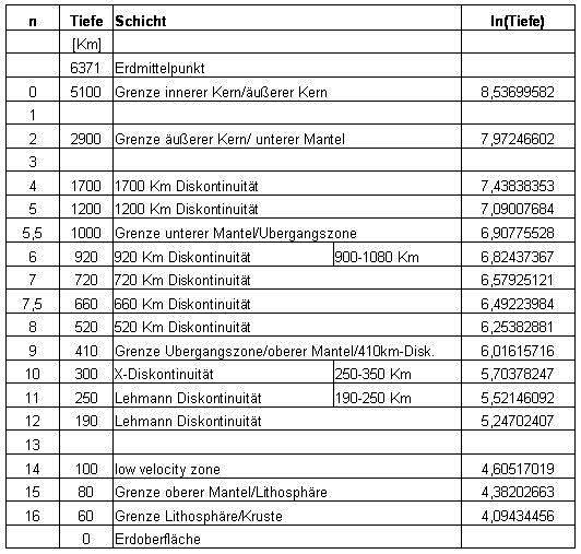
| The newly added layers in the numbering of 1 , 3 and 13 are # clear to see in the table. The corrected function looks like this: |
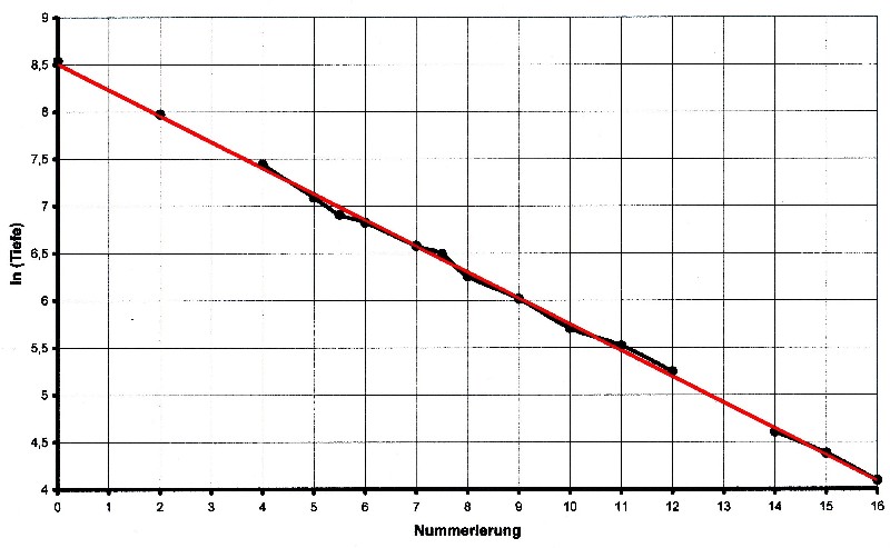
| Illustration 3.6.2 – linear regression |
| The red line in the illustration 3.6.2 represents a
linear function that was obtained by linear regression from the corrected table.
It is to see that the layer values match well with the approximation function. The following applies to the additive constant: b = ln wMax = ln Tn = ln 5100 = 8,536995 The following applies to the slope of the line: Δ y = ln wMax – ln wMin = ln 5100 – ln 60 = 4,442651 Δ x = n = 16 a = Δ y/Δ x = 4,442651/16 = 0,277665 A linear function for the geological layers can be used here as a solution approach. In general, the following applies to the straight line from Figure 3.6.2: : y = ln(depth) = –a·x + b The values found are inserted into the straight line equation: It results: ln(Tiefe) = – 0,2777 · x + 8,537 By rearranging you get: |
| 3.6.1 - Equation: | Tiefe = 5100 · e - 0,2777·x [Km] |
| Putting x = n then following function arises for equation 3.6.1: |
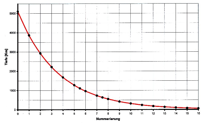
| Illustration 3.6.3 – depth of the geologic layers |
| Equation 3.6.1 has all of the properties that are necessary to 2.11.3, to come as a function of solution
of the Laplace equation into account. Thus the geological layers represent a solution of Laplace's
equation, specially of the radial component. In consequence this theorem can be set up: |
| 3.6.2 - Theorem: | The geological layers are an expression of an oscillation phenomenon. |
| On the equation 3.6.1 can be still made simplifications. It applies: 0,2777 = 3,6-1 = 5/18 SAll values ??used result in the equation for the depth of the geological shells: |
| 3.6.3 - Equation: |  |
[Km] |
| It can be made the following relationship: rik = RE/5 rik = inner core and RE= 6371 Km and it still applies: 5100 = RE– rik = 4/5 RE = 4rik Then, generally you can write: |
| 3.6.4 - Equation: |  |
[Km] |
| Then, you can write for the geological layers: |
| 3.6.5 - Equation: |  |
[Km] |
| The layers sorted by depth and the calculated values result in the following table: |
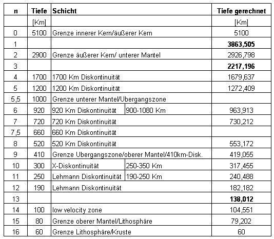
| The average error of the calculated values for the geological shells is less than 1 percent.. In addition, three more bowls are created. |
|
200 sides, 23 of them in color 154 pictures 38 tables Production und Publishing: ISBN 978-3-7357-3854-7 Price: 25 Euro |